Technical Details: BSGAL Training, Swin-L Backbone, and Dynamic Threshold Strategy

Table of Links

Abstract and 1 Introduction

1. Related work

   2.1. Generative Data Augmentation

   2.2. Active Learning and Data Analysis

2. Preliminary

3. Our method

   4.1. Estimation of Contribution in the Ideal Scenario

   4.2. Batched Streaming Generative Active Learning

4. Experiments and 5.1. Offline Setting

   5.2. Online Setting

5. Conclusion, Broader Impact, and References

   \

A. Implementation Details

B. More ablations

C. Discussion

D. Visualization

A. Implementation Details

A.1. Dataset

We choose LVIS (Gupta et al., 2019) as the dataset for our experiments. LVIS is a large-scale instance segmentation dataset, comprising approximately 160,000 images with over 2 million high-quality instance segmentation annotations across 1203 real-world categories. The dataset is further divided into three categories: rare, common, and frequent, based on their occurrence across images. Instances marked as ‘rare’ appear in 1-10 images, ‘common’ instances appear in 11-100 images, whereas ‘frequent’ instances appear in more than 100 images. The overall dataset exhibits a long-tail distribution, closely resembling the data distribution in the real world, and is widely applied under multiple settings, including few-shot segmentation (Liu et al., 2023) and open-world segmentation (Wang et al., 2022; Zhu et al., 2023). Therefore, we believe that selecting LVIS allows for a better reflection of the model’s performance in real-world scenarios. We use the official LVIS dataset splits, with about 100,000 images in the training set and 20,000 images in the validation set.

A.2. Data Generation

Our data generation and annotation process is consistent with Zhao et al. (2023), and we briefly introduce it here. We first use StableDiffusion V1.5 (Rombach et al., 2022a) (SD) as the generative model. For the 1203 categories in LVIS (Gupta et al., 2019), we generate 1000 images per category, with image resolution 512 × 512. The prompt template for generation is “a photo of a single {CATEGORY NAME}”. We use U2Net (Qin et al., 2020), SelfReformer (Yun and Lin, 2022), UFO (Su et al., 2023), and CLIPseg (Luddecke and Ecker ¨ , 2022) respectively to annotate the raw generative images, and select the mask with the highest CLIP score as the final annotation. To ensure data quality, images with CLIP scores below 0.21 are filtered out as low-quality images. During training, we also employ the instance paste strategy provided by Zhao et al. (2023) for data augmentation. For each instance, we randomly resize it to match the distribution of its category in the training set. The maximum number of pasted instances per image is set to 20.

\ In addition, to further expand the diversity of generated data and make our research more universal, we also use other generative models, including DeepFloyd-IF (Shonenkov et al., 2023) (IF) and Perfusion (Tewel et al., 2023) (PER), with 500 images per category per model. For IF, we use the pre-trained model provided by the author, and the generated images are the output of Stage II, with a resolution of 256×256. For PER, the base model we use is StableDiffusion V1.5. For each category, we fine-tune the model using the images croped from the training set, with 400 fine-tuning steps. We use the fine-tuned model to generate images.

\

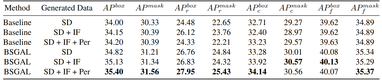
\ We also explore the effect of using different generated data on the model performance (see Table 7). We can see that based on the original StableDiffusion V1.5, using other generative models can bring some performance improvement, but this improvement is not obvious. Specifically, for specific frequency categories, we found that IF has a more significant improvement for rare categories, while PER has a more significant improvement for common categories. This is likely because IF data is more diverse, while PER data is more consistent with the distribution of the training set. Considering that the overall performance has been improved to a certain extent, we finally adopt the generated data of SD + IF + PER for subsequent experiments.

A.3. Model Training

Follow Zhao et al. (2023), We use CenterNet2 (Zhou et al., 2021) as our segmentation model, with ResNet-50 (He et al., 2016) or Swin-L (Liu et al., 2022) as the backbone. For ResNet-50, the maximum training iteration is set to 90,000 and the model is initialized with weights first pretrained on ImageNet-22k then finetuned on LVIS (Gupta et al., 2019), as Zhao

\

\ et al. (2023) did. And we use 4 Nvidia 4090 GPUs with a batch size of 16 during training. As for Swin-L, the maximum training iteration is set to 180,000 and the model is initialized with weights pretrained on ImageNet-22k, since our early experiments show that this initialization can bring a slight improvement compared to the weights trained with LVIS. And we use 4 Nvidia A100 GPUs with a batch size of 16 for training. Besides, due to the large number of parameters of Swin-L, the additional memory occupied by saving the gradient is large, so we actually use the algorithm in Algorithm 2.

\ The other unspecified parameters also follow the same settings as X-Paste (Zhao et al., 2023), such as the AdamW (Loshchilov and Hutter, 2017) optimizer with an initial learning rate of 1e−4.

A.4. Data Amount

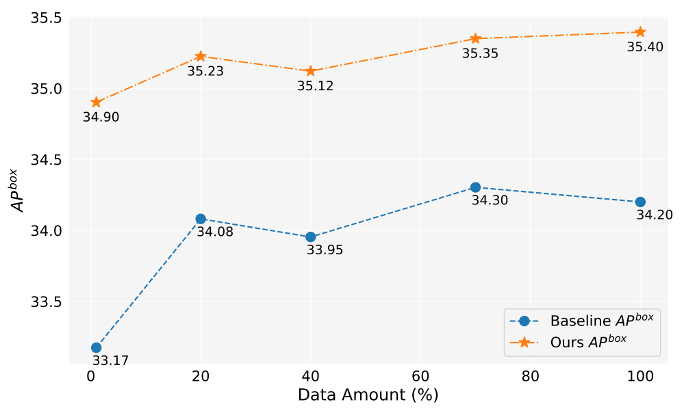
In this work, we have generated over 2 million images. Figure 5 shows the model performances when using different amount of generated data(1%,10%,40%,70%,100%). Overall, as the amount of generated data increases, the performance of the model also improves, but there is also some fluctuation. Our method is always better than the baseline, which proves the effectiveness and robustness of our method.

A.5. Contribution Estimation

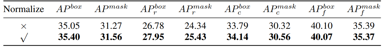
\ Thus, we essentially calculate the cosine similarity. Then we conducted an experimental comparison, as shown in Table 8,

\

\

\ we can see that if we normalize the gradient, our method will have a certain improvement. In addition, since we need to keep two different thresholds, it is difficult to ensure the consistency of the acceptance rate. So we adopt a dynamic threshold strategy, pre-set an acceptance rate, maintain a queue to save the contribution of the previous iter, and then dynamically adjust the threshold according to the queue, so that the acceptance rate stays at the pre-set acceptance rate.

A.6. Toy Experiment

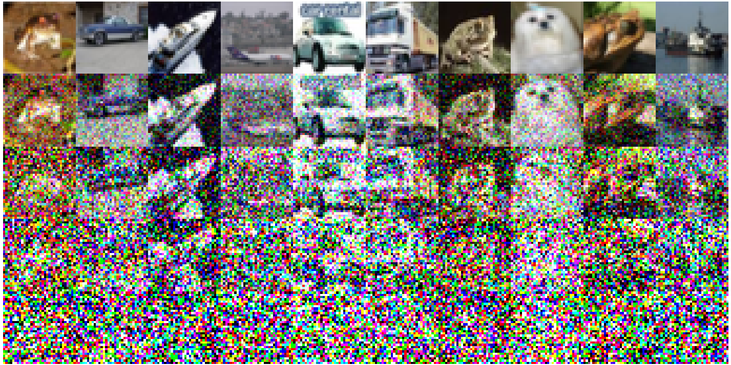
The following are the specific experimental settings implemented on CIFAR-10: We employed a simple ResNet18 as the baseline model and conducted training over 200 epochs, and the accuracy after training on the original training set is 93.02%. The learning rate is set at 0.1, utilizing the SGD optimizer. A momentum of 0.9 is in effect, with a weight decay of 5e-4. We use a cosine annealing learning rate scheduler. The constructed noisy images are depicted in Figure 6. A decline in image quality is observed as the noise level escalates. Notably, when the noise level reaches 200, the images become significantly challenging to identify. For Table 1, we use Split1 as R, while G consists of ‘Split2 + Noise40’, ‘Split3 + Noise100’, ‘Split4 + Noise200’,

A.7. A Simplification Only Forward Once

\

:::info Authors:

(1) Muzhi Zhu, with equal contribution from Zhejiang University, China;

(2) Chengxiang Fan, with equal contribution from Zhejiang University, China;

(3) Hao Chen, Zhejiang University, China ([email protected]);

(4) Yang Liu, Zhejiang University, China;

(5) Weian Mao, Zhejiang University, China and The University of Adelaide, Australia;

(6) Xiaogang Xu, Zhejiang University, China;

(7) Chunhua Shen, Zhejiang University, China ([email protected]).

:::

:::info This paper is available on arxiv under CC BY-NC-ND 4.0 Deed (Attribution-Noncommercial-Noderivs 4.0 International) license.

:::

\